Usage#
The package pyzernike is a Python package to compute Zernike polynomials and their derivatives.
Compute Zernike Polynomials#
To compute the Zernike polynomials \(Z_{n}^{m}\), use the following code:
from pyzernike import zernike_polynomial
import numpy as np

rho = np.linspace(0, 1, 100)
theta = np.linspace(0, 2*np.pi, 100)

n = 3
m = 1
result = zernike_polynomial(rho, theta, [n], [m])
Z_31 = result[0] # result is a list of Zernike polynomials for given n and m
To compute the second derivatives of the Zernike polynomials \(Z_{n,m}\) with respect to \(\rho\):
from pyzernike import zernike_polynomial
import numpy as np

rho = np.linspace(0, 1, 100)
theta = np.linspace(0, 2*np.pi, 100)

n = 3
m = 1
Z_31_drho_drho = zernike_polynomial(rho, theta, [n], [m], rho_derivative=[2])[0]
To compute several Zernike polynomials at once, you can pass lists of \(n\), \(m\), and their derivatives:
from pyzernike import zernike_polynomial
import numpy as np

rho = np.linspace(0, 1, 100)
theta = np.linspace(0, 2*np.pi, 100)

n = [3, 4, 5]
m = [1, 2, 3]
dr = [2, 1, 0]  # Derivatives with respect to rho for each Zernike polynomial
theta_derivative = [0, 1, 2]  # Derivatives with respect to theta for each Zernike polynomial

result = zernike_polynomial(rho, theta, n, m, rho_derivative=dr, theta_derivative=theta_derivative)

Z_31_drho_drho = result[0]  # Zernike polynomial for n=3, m=1 with second derivative with respect to rho
Z_42_drho_dtheta = result[1]  # Zernike polynomial for n=4, m=2 with first derivative with respect to theta and first derivative with respect to rho
Z_53_dtheta_dtheta = result[2]  # Zernike polynomial for n=5, m=3 with second derivative with respect to theta
See also
pyzernike.zernike_polynomial()for more details on the function parameters and usage.pyzernike.radial_polynomial()for computing radial polynomials.
Get the mathematical expression of Zernike Polynomials#
To get the mathematical expression of Zernike polynomials, you can use the zernike_symbolic function:
from pyzernike import zernike_symbolic

n = 3
m = 1
result = zernike_symbolic([n], [m])
expression = result[0]  # result is a list of symbolic expressions for given n and m
print(expression)  # This will print the symbolic expression of Zernike polynomial Z_31
Note
x is the symbol for \(\rho\) in the symbolic expression, and y is the symbol for \(\theta\).
You can use these symbols to manipulate the expressions further if needed.
import numpy
import sympy
rho = numpy.linspace(0, 1, 100)
theta = numpy.linspace(0, 2 * numpy.pi, 100)

# `x` represents the radial coordinate in the symbolic expression
# `y` represents the angular coordinate in the symbolic expression

func = sympy.lambdify(['x', 'y'], expression, 'numpy')
evaluated_result = func(rho, theta)
See also
pyzernike.zernike_symbolic()for more details on the function parameters and usage.pyzernike.radial_symbolic()for computing symbolic radial polynomials.
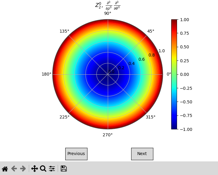
Display Zernike Polynomials#
To visualize the Zernike polynomials, you can use the zernike_display function. This function generates plots for the specified Zernike polynomials.
from pyzernike import zernike_display

n = [0, 1, 2, 3, 4]
m = [0, 1, -1, 2, -2]
zernike_display(n=n, m=m)
See also
pyzernike.zernike_display()for more details on the function parameters and usage.pyzernike.radial_display()for displaying radial Zernike polynomials.
Going Further with pyzernike#
Compute all Zernike polynomials up to a specified order#
To compute all Zernike polynomials up to a specified order, you can use the zernike_polynomial_up_to_order function. This function generates Zernike polynomials for all valid (n, m) pairs up to the given maximum order.
from pyzernike import zernike_polynomial_up_to_order, zernike_order_to_index
import numpy as np

rho = np.linspace(0, 1, 100)
theta = np.linspace(0, 2*np.pi, 100)

# Specify the maximum order
max_order = 4

# Compute all Zernike polynomials up to the specified order
result = zernike_polynomial_up_to_order(rho, theta, max_order)

# Extract the Zernike polynomials and their corresponding (n, m) orders
n = [2]
m = [0]
index = zernike_order_to_index(n, m)[0]  # Get the index for Z_20 (several (n, m) pairs can be provided)
Z_20 = result[index]  # Access the Zernike polynomial Z_20
See also
pyzernike.zernike_polynomial_up_to_order()for more details on the function parameters and usage.pyzernike.zernike_order_to_index()to convert (n, m) orders to their corresponding indices.pyzernike.zernike_index_to_order()to convert indices back to (n, m) orders.
Compute Zernike polynomials in an extended domain (e.g., Cartesian coordinates)#
To compute Zernike polynomials in Cartesian coordinates (x, y), you can use the xy_zernike_polynomial function. This function computes the Zernike polynomials over an extended domain \(G\).
For example, lets compute the Zernike polynomial \(Z_{3}^{1}\) in Cartesian coordinates over a radius of 2:
from pyzernike import xy_zernike_polynomial
import numpy as np

# Create a grid of (x, y) points over the extended domain G
x = np.linspace(-2, 2, 200)
y = np.linspace(-2, 2, 200)
X, Y = np.meshgrid(x, y)

n = [3]
m = [1]

# Compute the Zernike polynomial Z_31 in Cartesian coordinates extended over a radius of 2
result = xy_zernike_polynomial(X, Y, n, m, Rx=2, Ry=2)
Z_31_xy = result[0]  # result is a list of Zernike polynomials for given n and m
See also
pyzernike.xy_zernike_polynomial()for more details on the function parameters and usage.pyzernike.xy_zernike_polynomial_up_to_order()to compute all Zernike polynomials up to a specified order in an extended domain (e.g., Cartesian coordinates).
Command Line Display#
To display Zernike polynomials from the command line, you can use the pyzernike command followed by the desired options. For example:
pyzernike -r -n 3
This command will display the radial Zernike polynomials up to order 3.
To see the full list of options, you can run:
pyzernike --help
The available options are:
flag
-ror--radialwill display the radial Zernike polynomials instead of the full Zernike polynomials.flag
-n {N}or`--n {N}`will specify the maximum order of the Zernike polynomials to display. If not specified, the default value is 5flag
-dr {D}`or--rho_derivative {D}can be used to specify the radial derivative of the Zernike polynomials. If not specified, the default value is 0 for all polynomials.flag
-dt {D}`or--theta_derivative {D}can be used to specify the angular derivative of the Zernike polynomials. If not specified, the default value is 0 for all polynomials.flag
-ior--interactivecan be used to launch the interactive display window. If given, ignore other options and launch the interactive display.flag
-hor--helpcan be used to display the help message.