pyzernike.zernike_display

pyzernike.zernike_display(n: ~numpy.array | ~typing.Sequence[~numbers.Integral], m: ~numpy.array | ~typing.Sequence[~numbers.Integral], rho_derivative: ~numpy.array | ~typing.Sequence[~numbers.Integral] | None = None, theta_derivative: ~numpy.array | ~typing.Sequence[~numbers.Integral] | None = None, precompute: bool = True, float_type: ~numpy.floating = <class 'numpy.float64'>) → None

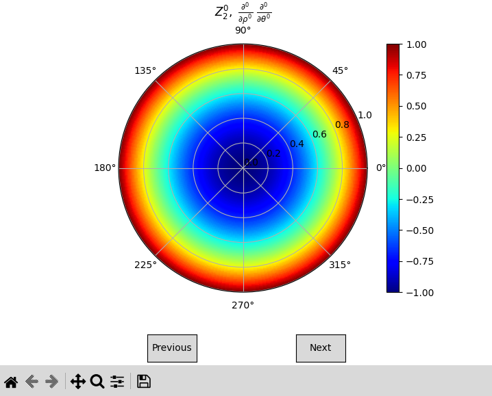
Display the Zernike polynomial \(Z_{n}^{m}(\rho, \theta)\) for \(\rho \leq 1\) and \(\theta \in [0, 2\pi]\) in an interactive matplotlib figure.

The Zernike polynomial is defined as follows:

\[Z_{n}^{m}(\rho, \theta) = R_{n}^{m}(\rho) \cos(m \theta) \quad \text{if} \quad m \geq 0\]

\[Z_{n}^{m}(\rho, \theta) = R_{n}^{-m}(\rho) \sin(-m \theta) \quad \text{if} \quad m < 0\]

If \(n < 0\), \(n < |m|\), or \((n - m)\) is odd, the polynomial is zero.

See also

• pyzernike.radial_display() for displaying the radial part of the Zernike polynomial \(R_{n}^{m}(\rho)\).

• pyzernike.core.core_display() to inspect the core implementation of the display.

• The page Mathematical description in the documentation for the detailed mathematical description of the Zernike polynomials.

The function allows to display several Zernike polynomials for different sets of (order, azimuthal frequency, derivative orders) given as sequences.

• The parameters n, m, rho_derivative and theta_derivative must be sequences of integers with the same length.

Parameters:

• n (Sequence[Integral] or numpy.array) – A sequence (List, Tuple) or 1D numpy array of the radial order(s) of the Zernike polynomial(s) to display. Must be non-negative integers.

• m (Sequence[Integral] or numpy.array) – A sequence (List, Tuple) or 1D numpy array of the azimuthal frequency(ies) of the Zernike polynomial(s) to display. Must be non-negative integers.

• rho_derivative (Optional[Union[Sequence[Integral], numpy.array]], optional) – A sequence (List, Tuple) or 1D numpy array of the order(s) of the radial derivative(s) to display. Must be non-negative integers. If None, is it assumed that rho_derivative is 0 for all polynomials.

• theta_derivative (Optional[Union[Sequence[Integral], numpy.array]], optional) – A sequence (List, Tuple) or 1D numpy array of the order(s) of the angular derivative(s) to display. Must be non-negative integers. If None, is it assumed that theta_derivative is 0 for all polynomials.

• precompute (bool, optional) – If True, the useful terms for the Zernike polynomials are precomputed to optimize the computation. If False, the useful terms are computed on-the-fly to avoid memory overhead. Default is True.

• float_type (numpy.floating, optional) – The floating point type to use for the computations. Default is numpy.float64.

Return type:

None

Raises:

• TypeError – If n, m, rho_derivative or theta_derivative (if not None) are not sequences of integers.

• ValueError – If the lengths of n, m, rho_derivative and theta_derivative (if not None) are not the same.

Examples

Display the Zernike polynomial \(Z_{2}^{0}(\rho, \theta)\):

from pyzernike import zernike_display
zernike_display(n=[2], m=[0]) # This will display the Zernike polynomial Z_2^0 in an interactive matplotlib figure.

To display multiple Zernike polynomials, you can pass sequences for n and m:

from pyzernike import zernike_display
zernike_display(n=[2, 3, 4], m=[0, 1, 2], rho_derivative=[0, 0, 1], theta_derivative=[0, 1, 0])